MLE Examples
These are a few examples of applying the MLE method to estimate unknown parameters in different distributions.
The likelihood function is shown, and by taking logs and differentiating the maximum likelihood estimator of the parameter is calculated.
The likelihood ratio and log likelihood function is then calculated for a hypothetical value of the parameter.
Binomial
See Binomial Distrubution .
L ( ~p ) _ = _ ( ^~n_~x ) ~p^~x ( 1 - ~p )^{~n - ~x}
l ( ~p ) _ #:= _ log_~e L ( ~p ) _ = _ log_~e( ^~n_~x ) + ~x log_~e ~p + (~n - ~x) log_~e( 1 - ~p )
l #' ( ~p ) _ #:= _ ( ~x ./ ~p ) - (~n - ~x) ./ ( 1 - ~p )
est{~p} _ = _ ~x ./ ~n
LR ( ~x ) _ = _ L ( ~p_0 ) ./ L ( est{~p} ) _ = _ ( ~n~p_0 ./ ~x ) ^~x # ((~n - ~n~p_0) ./ (~n - ~x)) ^{~n - ~x}
LL ( ~x ) _ = _ -2 log_~e LR ( ~x ) _ = _ -2 ~x log_~e ( ~n~p_0 ./ ~x ) - 2 ( ~n - ~x ) log_~e ((~n - ~n~p_0) ./ (~n - ~x))
_ _ _ _ _ _ = _ 2 ~x log_~e ( ~x ./ ~n~p_0 ) + 2 ( ~n - ~x ) log_~e ((~n - ~x) ./ (~n - ~n~p_0))
Geometric
See Geometric Distrubution .
L ( ~p ) _ = _ ~p ( 1 - ~p ) ^~x
l ( ~p ) _ #:= _ log_~e L ( ~p ) _ = _ log_~e ~p + ~x log_~e ( 1 - ~p )
l #' ( ~p ) _ = _ 1 ./ ~p _ - _ ~x ./ ( 1 - ~p )
est{~p} _ = _ 1 ./ ( ~x + 1 )
LR ( ~x ) _ = _ L ( ~p_0 ) ./ L ( est{~p} ) _ = _ ( ~x + 1 ) ~p_0 \{ ( ~x + 1 ) ( 1 - ~p_0 ) ./ ~x \} ^~x
LL ( ~x ) _ = _ -2 log_~e LR ( ~x ) _ = _ -2 \{ ( ~x + 1 ) log_~e ( ~x + 1 ) - ~x log_~e ~x + log_~e ~p_0 + ~x log_~e ( 1 - ~p_0 ) \}
Poisson
See Poisson Distrubution .
L ( &mu. ) _ = _ &mu.^~x e^{-&mu.} ./ ~x#!
l ( &mu. ) _ #:= _ log_~e L ( &mu. ) _ = _ ~x log_~e &mu. - &mu. - log_~e ~x#!
l #' ( &mu. ) _ = _ ~x ./ &mu. - 1
est{&mu.} _ = _ ~x
LR ( ~x ) _ = _ L ( &mu._0 ) ./ L ( est{&mu.} ) _ = _ &mu._0^~x e^{-&mu._0} ./ ~x^~x e^{-~x}
LL ( ~x ) _ = _ -2 log_~e LR ( ~x ) _ = _ 2 &mu._0 - 2 ~x ( log_e ( &mu._0 / ~x ) + 1 )
Normal
See Normal Distrubution .
L ( &mu. ) _ = _ fract{1,&sqrt.${2&pi.&sigma.&powtwo.}} exp rndb{fract{- ( ~x - &mu. )^2,2&sigma.&powtwo. }}
l ( &mu. ) _ #:= _ log_~e L ( &mu. ) _ = _ log_~e fract{1,&sqrt.${2&pi.&sigma.&powtwo.}} + rndb{fract{- ( ~x - &mu. )^2,2&sigma.&powtwo. }}
l #' ( &mu. ) _ = _ ( ~x - &mu. ) / &sigma.&powtwo.
est{&mu.} _ = _ ~x _ _ (This is obvious by just looking at the likelihood function.)
LR ( ~x ) _ = _ L ( &mu._0 ) ./ L ( est{&mu.} ) _ = _ exp rndb{fract{- ( ~x - &mu._0 )^2,2&sigma.&powtwo. }}
LL ( ~x ) _ = _ -2 log_~e LR ( ~x ) _ = _ fract{( ~x - &mu._0 )^2,&sigma.&powtwo. }
Exponential
 See Exponential Distrubution .
L ( &beta. ) _ = _ &beta. e^{- &beta.~x}
l ( &beta. ) _ #:= _ log_~e L ( &beta. ) _ = _ log_~e &beta. - &beta.~x
l #' ( &beta. ) _ = _ 1 ./ &beta. _ - _ ~x
est{&beta.} _ = _ 1 ./ ~x
LR ( ~x ) _ = _ L ( &beta._0 ) ./ L ( est{&beta.} ) _ = _ &beta._0 ~x e^{ 1 - &beta._0 ~x}
LL ( ~x ) _ = _ -2 log_~e LR ( ~x ) _ = _ 2 &beta._0 ~x - 2 log_~e &beta._0 ~x - 2

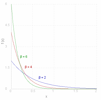
The graph on the left shows the exponential distribution for various &beta.. Note that the function with &beta. = 4 is the maximum one of these at the point ~x = 0.25.
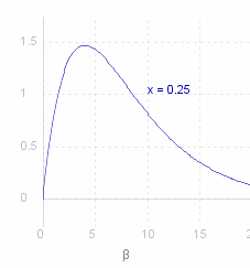
The graph on the right shows the same function, but this time with varying &beta. but ~x fixed at 0.25. As calculated above, this has maximum at &beta. = 4.
Source for the graphs shown on this page can be viewed by going to the diagram capture page .