Evaluating Integrals
Derivative Formula
If _ f , f ^{(1)}, f ^{(2)}, ... , f ^{(~n)} _ are all continuous on _ [ -~K, ~K ] _ then
f ( ~x ) _ _ _ = _ _ _ sum{fract{~x^{~r},~r#!} f ^{(~r)}(0),0,~n - 1} _ + _ R_~n ( ~x ) _ _ for | ~x | < ~K
where _ _ R_~n ( ~x ) _ = _ int{,0,~x,}fract{( ~x - ~t )^{~n - 1},( ~n - 1 )#!} f ^{(~n)}( ~t ) d~t
Proof:
To be provided
Simpson's Rule
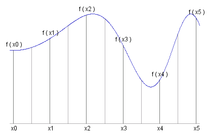
For any three points in the plane we can find a parabola of the form _ ~y = ~A~x^2 + ~B~x + ~C _ that passes through the three points. _ [Solve the three simultaneous equations _ ~y_~i = ~A~x_~i^2 + ~B~x_~i + ~C ].

Consider a continuous function _ f _ in the range [ -~h , ~h ] as shown in the diagram. _ The parabola _ ~y = ~A~x^2 + ~B~x + ~C _ passes through the points _ ( -~h , f ( -~h ) ) , _ ( 0 , f ( 0 ) ) , _ and _ ( ~h , f ( ~h ) ) .
So _ f ( -~h ) _ = _ ~A~h^2 - ~B~h + ~C , _ _ f ( 0 ) _ = _ ~C , _ _ and _ f ( ~h ) _ = _ ~A~h^2 + ~B~h + ~C ,
Then
int{f ( ~x ), -~h, ~h , d~x} _ _ ~= _ _ int{, -~h, ~h ,}~A~x^2 + ~B~x + ~C d~x _ = _ script{sqrb{fract{1,3}~A~x^3 + fract{1,2}~B~x^2 + ~C~x},,, ~h, -~h}
_ = _ fract{2,3}~A~h^3 + 2~C~h _ = _ fract{~h,3} ( 2~A~h^2 + 6~C ) _ = _ fract{~h,3} ( f ( ~h ) + 4 f ( 0 ) + f ( -~h ))
The error function is defined by:
E ( ~h ) _ _ #:= _ _ int{f ( ~x ), -~h, ~h , d~x} - fract{~h,3} ( f ( ~h ) + 4 f ( 0 ) + f ( -~h ))
E ( 0 ) _ = _ 0
differentiating with respect to ~h :
E^{(1)}( ~h ) _ = _ f ( ~h ) _ + _ f ( -~h ) _ - _ fract{ 1 , 3 } ( f ( ~h ) + 4 f ( 0 ) + f ( -~h )) _ - _ fract{ ~h , 3 } ( f '( ~h ) - f '( -~h ) )
_ = _ fract{ 2 , 3 } f ( ~h ) _ + _ fract{ 2 , 3 } f ( -~h ) _ - _ fract{ 4 , 3 } f ( 0 ) _ - _ fract{ ~h , 3 } ( f '( ~h ) _ - _ f '( -~h ) )
E^{(1)}( 0 ) _ = _ 0
[Note: by fundamental theorem _ ~{∫}_{-~h}^~h f ( ~x ) d~x _ = _ F ( ~h ) - F ( -~h ) , _ where _ f = F ' , differentiating we get _ f ( ~h ) + f ( -~h ) .]
E^{(2)}( ~h ) _ = _ fract{ 2 , 3 } f '( ~h ) - fract{ 2 , 3 } f '( -~h ) - fract{ 1 , 3 } ( f '( ~h ) - f '( -~h ) ) - fract{ ~h , 3 } ( f ^{(2)}( ~h ) + f ^{(2)}( -~h ) )
_ = _ fract{ 1 , 3 } f '( ~h ) _ - _ fract{ 1 , 3 } f '( -~h ) _ - _ fract{ ~h , 3 } ( f ^{(2)}( ~h ) _ + _ f ^{(2)}( -~h ) )
E^{(2)}( 0 ) _ = _ 0
E^{(3)}( ~h ) _ = _ fract{ 1 , 3 } f ^{(2)}( ~h ) + fract{ 1 , 3 } f ^{(2)}( -~h ) - fract{ 1 , 3 } ( f ^{(2)}( ~h ) + f ^{(2)}( -~h ) ) - fract{ ~h , 3 } ( f ^{(3)}( ~h ) - f ^{(3)}( -~h ) )
_ = _ - fract{ ~h , 3 } ( f ^{(3)}( ~h ) - f ^{(3)}( -~h ) )
So by the mean value theorem
E^{(3)}( ~h ) _ = _ - fract{ 2~h^2 , 3 } f ^{(4)}( &xi. ) , _ _ _ _ some _ &xi. &in. ( -~h , ~h )
Suppose _ f ^{(4)} _ is bounded in ( -~h , ~h ) . _ I.e. _ | f ^{(4)}( &xi. ) | _ =< _ ~M , _ &xi. &in. ( -~h , ~h ) , _ then
_ _ _ _ _ -(2/3) ~h^2 ~M _ =< _ E^{(3)}( ~h ) _ =< _ (2/3) ~h^2 ~M
so
_ _ _ _ _ -(2/3) ~M ~{∫}_0^~h ~x^2 d~x _ =< _ ~{∫}_0^~h E^{(3)}( ~x ) d~x _ =< _ (2/3) ~M ~{∫}_0^~h ~x^2 d~x
_
_ _ _ _ _ -(2/9) ~h^3 ~M _ =< _ E^{(2)}( ~h ) _ =< _ (2/9) ~h^3 ~M _ _ _ [Recall: _ E^{(2)}( 0 ) _ = _ 0 ]
Continuing to integrate from 0 to ~h :
_ _ _ _ _ -(1/18) ~h^4 ~M _ =< _ E^{(1)}( ~h ) _ =< _ (1/18) ~h^4 ~M _ _ _ [ E^{(1)}( 0 ) _ = _ 0 ]
_ _ _ _ _ -(1/90) ~h^5 ~M _ =< _ E ( ~h ) _ =< _ (1/90) ~h^5 ~M _ _ _ [ E ( 0 ) _ = _ 0 ]
So we have
int{f ( ~x ), -~h, ~h , d~x} _ _ ~= _ _ fract{~h,3} ( f ( ~h ) + 4 f ( 0 ) + f ( -~h ))
With an error _ E ( ~h ) _ =< _ | (1/90) ~h^5 ~M | , _ _ where ~M is the upper bound on _ f ^{(4)} _ in ( -~h , ~h )
Generalising ( by simple translation )
int{f ( ~x ), ~c - ~h, ~c + ~h , d~x} _ _ ~= _ _ fract{~h ,3} rndb{ f ( ~c + ~h ) + 4 f ( ~c ) + f ( ~c - ~h ) }
or
int{f ( ~x ), ~a, ~b , d~x} _ _ ~= _ _ fract{~b - ~a,6} rndb{ f ( ~b ) + 4 f ( fract{~b + ~a,2} ) + f ( ~a ) }
The estimate is more accurate if we split the interval up into ~n equal sub-intervals, each of length 2~h ( i.e. ~h = ( ~b - ~a ) / 2~n ) and make the estimate for each sub-interval:
int{f ( ~x ), ~a, ~b , d~x} _ _ ~= _ _ sum{fract{~x_~i - ~x_{~i - 1},6} rndb{ f ( ~x_~i ) + 4 f ( fract{~x_~i + ~x_{~i - 1},2} ) + f ( ~x_{~i - 1} ) },~i = 1, ~n}
I.e. when the intervals are equal:
|
int{f ( ~x ), ~a, ~b , d~x} _ _ ~= _ _ fract{~b - ~a,6~n} sum{rndb{ f ( ~x_~i ) + 4 f ( fract{~x_~i + ~x_{~i - 1},2} ) + f ( ~x_{~i - 1} ) },~i = 1, ~n} |
With a bound on the error _ E _ =< _ | (1/90) ( ( ~b - ~a ) / 2~n )^5 ~M | _ = _ | (1/2880) ( ( ~b - ~a ) / ~n )^5 ~M | , _ _ where ~M is the upper bound on _ f ^{(4)} _ in ( ~a , ~b )
#{Example}:
This example is taken from Stephenson p235.
"Evaluate the integral
~I _ _ = _ _ int{,0,&pi./2,}fract{d&theta.,&sqrt.${ 1 - 1/2 sin&powtwo. &theta. }}
using Simpson's rule with five ordinates."
The integral is evaluated using the #~{zSimpsonPrint ( )} function from the ~{MathymaDistr} package:
. . .
[Note that five ordinates equates to two sub intervals, the end- and mid- points of each sub-interval being ordinates.] Here is the output:
Integral Test
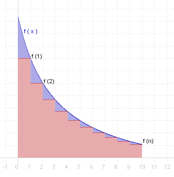
Let _ f _ be a positive decreasing function defined on [ 0 , &infty. ). _ As the diagram indicates
_ _ _ _ _ &sum._1^~n f ( ~x ) _ < _ ~{∫}_0^~n f ( ~x ) d~x _ _ [ _ < _ &sum._0^{~n-1} f ( ~x ) _ ]
The series _ &sum._1^~n f ( ~x ) _ is convergent _ _ <=> _ _ ~{∫}_0^~n f ( ~x ) d~x _ is bounded.
Or more generally:
_ _ _ _ _ &sum._~m^~n f ( ~x ) _ is convergent _ _ <=> _ _ ~{∫}_~m^~n_{- 1} f ( ~x ) d~x _ is bounded.