Calculating MLE statistics

We will look at calculating some of the MLE statistics such as significance probability for the binomial model. Some of the calculations will be specific to the binomial distribution, but the principles should be applicable to other distributions which we will deal with later, including continuous distributions such as the Normal.

Significance Probability

The difficulty in calculating the SP is deciding which values to include, i.e. which values have a likelihood ratio less than or equal to the test value. For the time being we'll concentrate on the binomial distribution. Obviously any value which is further from the maximum on the same side as the test value should be included, but where is the cut-off for values on the opposite side?

In the binomial distribution, if the hypothetical value of &theta. is 0.5, then the distribution is symmetric about ~n/2 and so is the likelihood ratio, so if the test value ~x < ~n/2 all values ~y =< ~x and ~y >= ~n - ~x are included. Include all ~y =< ~n - ~x and ~y >= ~x if ~x > ~n/2. (If ~x = n/2 then SP = 100%)

If &theta. is not 0.5 then the distribution and the likelihood ratio are no longer exactly symmetric.

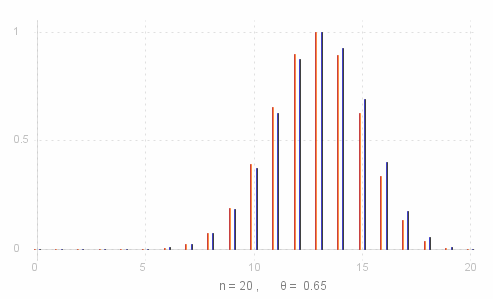
Take a look at the graphs on the right of the likelihood ratio function (red pins on the left) and the binomial probability function (normalised for comparison - blue pins on the right) for ~n = 20 and &theta. = 0.65.

Suppose our test value is 11, then if we consider the curves "almost" symmetric about ~n&theta. = 13, we would include all ~y =< 11 and ~y >= 15. This turns out to be OK as we can see from the graph that LR(15) < LR(11).

[ Note that _ LR(15) < LR(11) _ even though _ P(15; 20, 0.65) > P(11; 20, 0.65) ). So we cannot use the probability distribution as an exact guide to the likelihod ratio. ]

For the hypothesis H: &theta. = 0.65

SP(~x = 11) _ = _ p(~y | ~y =< 11 or ~y >= 15) = 0.2376 + 0.2454 _ = _ 0.4830 _ or _ 48.3%

However, if the test value were 15, then we would expect by symmetry arguments to use the same ~y, but as we have seen LR(11) < LR(15), so ~y = 11 should not be included.

SP(~x = 15) _ = _ p(~y | ~y =< 10 or ~y >= 15) = 0.1218 + 0.2454 _ = _ 0.3672 _ or _ 36.72%

So to calculate the ~{exact} SP, we need to calculate the likelihood ratio of the values on the opposite side of the curve until we find one that is less than or equal to the likelihood ratio of the test value.

Log Likelihood Function

So as we've just seen the SP is the sum of probabilities of all the values ~y for which LR(~y) =< LR(~x) where ~x is the result value.

We dont actually need the values of LR(~y) in the calculation, just their relative size. Now as log is a strictly increasing function we have that

LR(~y) < LR(~x) _ <=> _ log( LR(~y) ) < log( LR(~x) )

LR(~y) = LR(~x) _ <=> _ log( LR(~y) ) = log( LR(~x) )

Now _ 0 =< LR(~x) =< 1 , _ so log( LR(~x) ) will be zero or negative. So instead of working directly with log( LR(~x) ) it is conventional to work with the quantity -2 log( LR(~x) ). This is known as the #~{log likelihood} function of ~x, LL(x).

For the binomial distribution with parameters ~n and &theta.:

LL(~x) _ = _ -2 log( LR(~x) ) _ = _ -2 log rndb{script{rndb{fract{~n &theta._0,~x}},,,~x,} script{rndb{fract{~n ( 1 - &theta._0 ),~n - ~x}},,,~n - ~x,}}

_ _ _ _ _ _ = _ -2~x ( log ~n&theta. - log ~x ) - 2(~n - ~x) ( log (~n - ~n&theta.) - log (~n - ~x) )

And we can define the significance probability in terms of the log likelihood:

SP ( ~x ) _ = _ P\{ ~y | LL(~y) >= LL(~x) \}

Where the log likelihood function is really useful is in the Chi-squared test for the binomial model.

Distribution of MLE Statistics

Consider again the definition of the significance probability:

SP ( ~x ) _ = _ P\{ ~y | LR(~y) =< LR(~x) \}

Now the likelihood ratio function is just a function of the random variable ~X, so

SP(~x) _ = _ F_{LR} ( LR(~x) )

where F_{LR} is the (cummulative) distribution function for LR(~X), or similarly:

SP(~x) _ = _ P\{ ~y | LL(~y) >= LL(~x) \} _ = _ 1 - F_{LL} ( LL(~x) ) + P\{ ~y | LL(~y) = LL(~x) \}

where F_{LL} is the distribution function for Log-likelihood LL( ~X ). In the binomial model, where the number of trials, ~n , is large then P\{ ~y | LL(~y) = LL(~x) \} becomes very small, so we can write

SP(~x) _ ~~ _ 1 - F_{LL} ( LL(~x) )

So we would have a quick method of working out the significance probability for a binomial model if we had an expression for the distribution of the log-likelihood function of ~X. We will return to this line of thought when we look at the chi-squared test .

---