Central Forces
Motion Under A Central Force
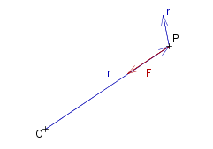 Consider the motion of a particle at P ( position vector #~r ) moving under the influence of a force #~F always directed towards the same point O (which we will adopt as the origin). The equation of motion is
~#F _ = _ ~m deriv2{#~r}
Then deriv2{#~r} is also parallel to ~#r, so _ ~#r # deriv2{#~r} _ = _ 0 . _ So
fract{d ( ~#r # deriv{#~r} ), d~t} _ = _ deriv{#~r} # deriv{#~r} + ~#r # deriv2{#~r} _ = _ 0 + 0 _ = _ 0
So _ _ _ _ _ _ ~#r # deriv{#~r} _ = _ ~{constant} _ =#: _ #~h
This means that ~#r and deriv{#~r} must always be in the plane perpendicular to #~h.
Motion In A Plane
We set up a system of rectangular coordinates such that the center of attraction O is the origin, and the ~x~y-plane coincides with the plane of motion (which contains ~#r and deriv{#~r}). The ~x-axis is the line from the origin O to the initial position .
_
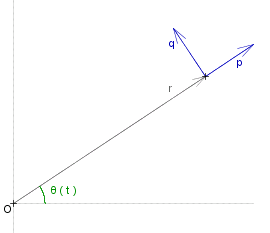 Let &theta. be the angle between #~r and the ~x-axis. &theta. changes with time of course.
We now introduce two unit vectors, #~p which is parallel to #~r, and #~q, which is perpendicular to #~r in the plane of motion ( i.e. the planeperpendicular to #~h ).
#~p _ = _ cos &theta. #~i + sin &theta. #~j
#~q _ = _ - sin &theta. #~i + cos &theta. #~j
It is easy to see that
deriv{#~p} _ = _ deriv{&theta.} #~q _ _ _ and _ _ _ deriv{#~q} _ = _ - deriv{&theta.} #~p
We have:
#~r _ = _ | ~#r | #~p _ = _ ~r #~p
deriv{#~r} _ = _ deriv{~r} #~p + ~r deriv{#~p} _ = _ deriv{~r} #~p + ~r deriv{&theta.} #~q
deriv2{#~r} _ = _ deriv2{~r} #~p + deriv{~r} deriv{#~p} + deriv{~r} deriv{&theta.} #~q + ~r deriv2{&theta.} #~q + ~r deriv{&theta.} deriv{#~q}
_ _ _ _ = _ ( deriv2{~r} - ~r ( deriv{&theta.} )^2 ) #~p _ + _ ( 2 deriv{~r} deriv{&theta.} + ~r deriv2{&theta.} ) #~q
Area Swept
We saw that
#~r # deriv{#~r} _ = _ ~{constant vector} _ =#: _ ~#h
In terms of #~p and #~q
~r #~p # ( deriv{~r} #~p + ~r deriv{&theta.} #~q ) _ = _ #~h _ => _ ~r^2 deriv{&theta.} ( #~p # #~q ) _ = _ #~h
and since #~p and #~q are unit vectors, and putting _ ~h _ #:= _ | #~h |
|
~r^2 deriv{&theta.} _ = _ ~h _ = _ ~{constant} |
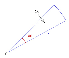
Let &delta.~A represent the area swept out in a small time interval &delta.~t. There will be a small change &delta.&theta. in the angle, so the area is approximately the area of the segment (see diagram right):
&delta.~A _ ~~ _ fract{~r^2&delta.&theta.,2} _ _ => _ _ fract{&delta.~A,&delta.~t} _ ~~ _ fract{~r^2,2} fract{&delta.&theta.,&delta.~t}
In the limit we have
fract{d~A,d~t} _ = _ fract{~r^2,2} fract{d&theta.,d~t}
|
deriv{~A} _ = _ ~h ./ 2 _ = _ ~{constant} ~A _ = _ ~~h ~t ./ 2 + ~{integration constant} |
Orbital Equation
Now _ deriv2{#~r} is parallel to ~#p , i.e. so
deriv2{#~r} _ = _ - ~a ~#p + 0 #~q
where _ ~a _ #:= _ | #~F | ./ ~m _ = _ | deriv2{#~r} | _ (i.e. the acceleration or force per unit mass). _ But
deriv2{#~r} _ = _ ( deriv2{~r} - ~r ( deriv{&theta.} )^2 ) #~p _ + _ ( 2 deriv{~r} deriv{&theta.} + ~r deriv2{&theta.} ) #~q
so by equating coefficients we have:
deriv2{~r} - ~r ( deriv{&theta.} )^2 _ = _ - ~a _ _ _ _ _ (#A)
2 deriv{~r} deriv{&theta.} + ~r deriv2{&theta.} _ = _ 0 _ _ _ _ _ (#B)
So far the equations of motion involve ~r and &theta. and their derivatives with respect to time. We will now eliminate the time factor to derive an equation purely in polar coordinates.
Put _ ~u _ #:= _ ~r^{-1} , then _ deriv{&theta.} _ = _ ~u^2 ~h , _ and
deriv{~r} _ = _ fract{d ~u^{-1},d ~t} _ = _ - ~u^{-2} fract{d ~u,d ~t} _ = _ - ~u^{-2} fract{d ~u,d &theta.} fract{d &theta.,d ~t} _ = _ - ~u^{-2} fract{d ~u,d &theta.} ~u^2 ~h
so _ deriv{~r} _ = _ - ~h ( d ~u ./ d &theta. ) , _ and
deriv2{~r} _ = _ - ~h fract{d,d ~t}rndb{fract{d ~u,d &theta.}} _ = _ - ~h fract{d,d &theta.}rndb{fract{d ~u,d &theta.}} # fract{d &theta.,d ~t} _ = _ - ~u^2 ~h ^2 fract{d ^2 ~u,d &theta. ^2}
So substituting for deriv2{~r}, ~r, and deriv{&theta.} in (#A) above
- ~u^2 ~h ^2 fract{d ^2 ~u,d &theta. ^2} _ - _ ~u^{-1} ~u^4 ~h^2 _ = _ - ~a
|
fract{d ^2 ~u,d &theta. ^2} _ + _ ~u _ = _ fract{ _ ~a _ ,~u^2 ~h ^2} |
This second degree differential equation links ~u ( = ~r^{-1} ) to the angle &theta., dependant on ~a = ~a(~t). It describes the ~#{orbit} taken by the paritcle and we will refer to it as the #~{orbital equation}.
Source for the graphs shown on this page can be viewed by going to the diagram capture page .