Functions of Joint Random Variables

Function of Two Random Variables

~X, ~Y are random variables and _ ~Z = &phi. ( ~X , ~Y ) , _ where _ &phi. #: &reals.^2 -> &reals. . _ Then ~Z is a random variable and its distribution function is

F_~Z ( ~z ) _ = _ ~{&integ.}~{&integ.}__{~A_~z} f_{~X,~Y} ( ~x , ~y ) d~x d~y

where _ ~A_~z = \{ ( ~x , ~y ) | &phi. ( ~x , ~y ) =< ~z \}

Sum of Two Random Variables

Sum of Real-Valued Random Variables

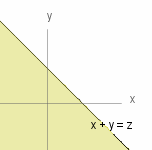
~Z = ~X + ~Y , _ ~A_~z = \{ ( ~x , ~y ) | ~x + ~y =< ~z \} . _ ~A_~z is the shaded area in the diagram on the right.

F_~Z ( ~z ) _ = _ ~{&integ.}__{-&infty.}^^{&infty.} ~{&integ.}__{-&infty.}^^{~z - ~x} f_{~X,~Y} ( ~x , ~y ) _ d~y d~x

_ _ _ _ _ = _ ~{&integ.}__{-&infty.}^^~z ~{&integ.}__{-&infty.}^^{&infty.} f_{~X,~Y} ( ~u , ~v - ~u ) _ d~u d~v

using the change of variable _ ~x = ~u , _ ~y = ~v - ~u , _ the Jacobian is 1 , _ and then changing the order of integration.

By definition _ F_~Z ( ~z ) _ = _ ~{&integ.}__{-&infty.}^^~z _ f_~Z ( ~v ) _ d~v , _ so

f_{~X + ~Y} ( ~v ) _ = _ ~{&integ.}__{-&infty.}^^{&infty.} f_{~X,~Y} ( ~u , ~v - ~u ) _ d~u

Sum of Non-Negative Random Variables

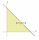
If ~X > 0 and ~Y > 0 then _ ~A_~z is the shaded area shown in the top diagram on the right.

F_~Z ( ~z ) _ = _ ~{&integ.}__0^^~z ~{&integ.}__0^^{~z - ~x} f_{~X,~Y} ( ~x , ~y ) _ d~y d~x

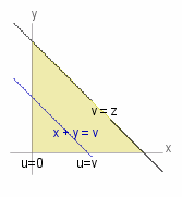
_ _ _ _ _ = _ ~{&integ.}__0^^~z ~{&integ.}__0^^~v f_{~X,~Y} ( ~u , ~v - ~u ) _ d~u d~v

using the same change of variables as above - see diagram bottom right for limits of integrals.

f_{~X + ~Y} ( ~v ) _ = _ ~{&integ.}__0^^~v f_{~X,~Y} ( ~u , ~v - ~u ) _ d~u

Sum of Independent Random Variables

If ~X and ~Y are independent then _ f_{~X + ~Y} ( ~z ) _ = _ ~{&integ.}__{-&infty.}^^{&infty.} _ f_~X ( ~x ) f_~Y ( ~z - ~x )_ d~x

or, if ~X, ~Y are also non-negative _ _ f_{~X + ~Y} ( ~z ) _ = _ ~{&integ.}__0^^~z _ f_~X ( ~x ) f_~Y ( ~z - ~x )_ d~x

#{Example}

#{1)} If ~X and ~Y are independent chi-squared distributed with one degree of freedom.

f_{~X + ~Y} ( ~z ) _ = _ int{,0,~z,,} fract{ e ^{-~x/2}, &sqrt.${2&pi.~x}} fract{ e ^{- ( ~z - ~x ) ./ 2},&sqrt.${2&pi.( ~z - ~x )}} _ d~x _ = _ fract{e ^{-~z/2}, 2&pi.} int{,0,~z,,} ~x^{- 1/2 } ( ~z - ~x )^{- 1/2 } _ d~x

#{2)} If ~X and ~Y are independent standard normally distributed , _ ~X ~ N ( 0 , 1 ) , _ ~Y ~ N ( 0 , 1 ).

f_{~X + ~Y} ( ~v ) _ = _ int{,-&infty.,&infty.,} _ fract{1,&sqrt.${2&pi.}} exp rndb{fract{- ~x^2,2}} fract{1,&sqrt.${2&pi.}} exp rndb{fract{- ( ~v - ~x )^2,2}} _ d~x

_ _ _ _ _ = _ fract{1,2&pi.} int{,-&infty.,&infty.,} _ exp rndb{fract{- ( ~x^2 + (~v - ~x )^2 ),2}} _ d~x

Note that _ ~x^2 + (~v - ~x )^2 _ = _ 2 ~x^2 + ~v^2 - 2 ~x ~v _ = _ 2 ( ~x - ~v/2 )^2 + ~v^2/2 .

Putting _ ~y _ = _ &sqrt.$2 ( ~x - ~v/2 ) , _ so _ d~y ./ d~x _ = _ &sqrt.$2 , _ and using this change of variable:

f_{~X + ~Y} ( ~v ) _ = _ fract{1,2&pi.} fract{1,&sqrt.$2} exp rndb{fract{- ~v^2 ,4}} _ int{,-&infty.,&infty.,} exp rndb{fract{- ~y^2 ,2}} _ d~y

_ _ _ _ _ = _ fract{1,&sqrt.${2&pi.}} fract{1,&sqrt.$2} exp rndb{fract{- ~v^2 ,4}} , _ _ _ Using the result : _ ~{&integ.}__{-&infty.}^^{&infty.} exp ( - ~y^2 ./ 2 ) d~y _ = _ &sqrt.${2&pi.}

So _ ~X + ~Y _ ~ _ N ( 0, 2 ) , _ _ ( i.e. &sigma.&powtwo. = 2 )

---