Simple Linear Regression

Simple Linear Regression Model

The simple linear regression model is one of the form:

Simple Linear Regression

To illustrate these methods, we will consider an experiment to determine what influences the abrasion coefficient of rubber. The abrasion (in ) is measured on 30 samples, together with the hardness (in ). The samples are also categorised by Strength, as "high" and "low" depending on whether Strength is greater than 22.3 (high) or less than or equal to 22.3 (low).

[This data is from O. L. Davies, Statistical Methods in Research and Production (Oliver & Boyd, 1972), and is quoted in Open University course M345 - Statistical Methods (The Open University, 1986)]

In this example, Abrasion is the response variable and Hardness is the only explanatory variable. This is known as a "simple linear regression" model We might be interested in proposing the model:

To set this model up in MathymaStats, we use the mathyma.stats.DataBlock method Model:

   var wModel = abrasionData.Model("Abrasion=_c+Hardness");

The "_c" term tells MathymaStats that we require a constant term in the model, corresponding to the a in the equation above. Leaving this out would mean that the model specified that the regression line goes through the origin, i.e:

Once our model has been defined, we would like to print some statistics and get estimates for the unknown parameters, a, b, and v. To do this use the cModel method Display, here is the full example (note the modules included in the < head > section):

< script type="text/javascript" src="../Lib/MathymaStat.js" >< /script >
< script type="text/javascript" src="../Lib/MathymaLinMod.js" >< /script >
< script type="text/javascript" src="../Lib/MathymaMatrix.js" >< /script >
< script type="text/javascript" src="../Lib/MathymaDistr.js" >< /script >
. . .
< script >
   var abrasionData = new mathyma.stats.DataBlock("StatsData/Abrasion.xml");
   abrasionData.ViewXML();
   abrasionData.AddVariables("Abrasion=ABR;Hardness=HNESS");
   var wModel = abrasionData.Model("Abrasion=_c+Hardness");
   wModel.Display();
< /script >

This is the output:

The significance probability is that for the hypothesis that the model reduces to the constant model:

"Root MS Error" is an estimate for the standard deviation for the model.

The second table lists the estimates for the parameters, the intercept (constant value) and the slope. The t-vale for the slope is the Student's t-test value for the hypothesis slope = 0. This has the same number of degrees of freedom as the residual, and is an alternative form of testing for zero slope. Note that the F-value is the square of the t-value. In fact the two tests are equivalent, as the square of a Student's t-distributed variable with n degrees of freedom is just an F-distributed variable with (1, ~n) degrees of freedom. The t-test comes into it's own when there are several slope variables (see Two Explanatory Variables)

The "Mean Response" is simply the mean of the response variable for the observations considered.

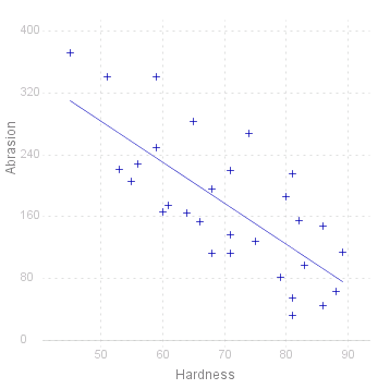
You can use the mathyma.stats.DataBlock method Plot to get a graphical view of the data:

< script >
   abrasionData.Plot("Abrasion:Hardness",true);
< /script >

Linear Regression by Group

Consider now the same set of observations, but this time they are split up into two groups by the factor STRENGTH. This factor has to be added to the mathyma.stats.DataBlock and then we can define a new model:

< script >
   abrasionData.AddFactors("STRENGTH=STRENGTH:low,180,high");
   var wModel2 = abrasionData.Model("Abrasion=_c+Hardness/STRENGTH");
   wModel2.Display();
< /script >

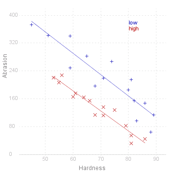
For a visualisation of the model we can use the Plot method:

< script >
   abrasionData.Plot("Abrasion:Hardness/STRENGTH",true);
< /script >

Comparing Slopes

An obvious question to ask in the above model is: "Are the two slopes the same?"

The model for the grouped data with two slopes is:

Two Explanatory Variables

We will now consider the same data, but instead of strength just being categorised as high or low we have the actual values. This is in a new file, so we start a new data block:

< script >
   abrasionData.AddVariables("Strength=STRENGTH");
   var wMod2Var = abrasionData.Model("Abrasion=_c+Hardness+Strength");
   wMod2Var.Display();
   abrasionData.Plot("Abrasion:Hardness",true);
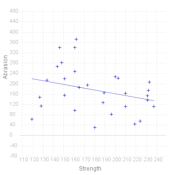
   abrasionData.Plot("Abrasion:Strength",true);
< /script >

Note that the two plots do not have the same vertical scale (this would amount to taking two projections of the same 3-D graph, Mathyma can't do this - yet!!)

The F-value now tests whether both slopes are zero - i.e. the plane of regression is totally horizontal, this does not seem to be the case.

To test the individual slopes we can check the t-values in the table of coefficients. Hardness has a t-value of -11.27, and Strength -7.073, both with very low significance probability, giving very little indication of either parameter being zero.

Model Reduction

Suppose, given the model with two explanatory variables that we want to test to see if a model with just one of the explanatory variables is good enough. This is a case of Model Reduction.

E.g. in this case suppose we want to see what happens if we remove Strength as an explanatory variable. This will result in the model we showed in Simple Linear Regression above, and is equivalent to testing for zero slope for Strength. This seems unlikely, as the significance probability for the t-value was very low, but we will go through with it for illustrative purposes.

First we display the two variable model again, then we define and display the reduced model (we can't use the simple linear regression data as this was in another file), then we do the model reduction test:

< script >
   wMod2Var.Display();
   var wMod1Hrd = abrasionData.Model("Abrasion=_c+Hardness");
   wMod1Hrd.Display();
   abrasionData.ModelReduction(wMod2Var, wMod1Hrd);
< /script >

What happens in going to the "reduced" model is that part of the sum of squares and degrees of freedom is lost from the model to the residual, so that the residual variation now becomes larger. Note that the total sum of squares and degrees of freedom is the same in the original and the reduced model.

Note that the F-value is the square of the t-value for the coefficient of slope of Strength in the original model, in fact the two tests are completely equivalent, as stated above, the square of an n d.f. Student's t-variable is a (1, n) d.f. F-variable.