Multi-variate Statistics

On this page we will demonstrate the graphical methods of investigating multivariate data. More complicated relationships between variables can be investigated using the methods of simple and multiple linear regression

To illustrate the methods provided by MathymaStats to investigate multi-variate data, we will consider an experiment to determine what influences the abrasion coefficient of rubber. The abrasion (in ) is measured on 30 samples, together with the hardness (in ). The samples are also categorised by Strength, as "high" and "low" depending on whether Strength is greater than or equal to 180 (high) or less than 180 (low).

[This data is from O. L. Davies, Statistical Methods in Research and Production (Oliver & Boyd, 1972), and is quoted in Open University course M345 - Statistical Methods (The Open University, 1986)]

Summarizing the data

To get basic statistics on any variable the mathyma.stats.DataBlock method "Summary" is used:

< script type="text/javascript" src="../Lib/MathymaStat.js" >< /script >
. . .
< script >
   var myData = new mathyma.stats.DataBlock("StatsData/Abrasion.xml");
   myData.ViewXML();
   myData.AddVariables("Abrasion=ABR;Hardness=HNESS;");
   myData.AddFactors("STRENGTH=STRENGTH:LOW,180,HIGH");
   myData.Summary("Abrasion");
   myData.Summary("Hardness");
< /script >

This produces the following output:

Bi-variate Plots

The mathyma.stats.DataBlock method "Plot" allows you to produce a variety of graphical output illustrating the data. Taking the above example on rubber abrasion, there are two variables, "Abrasion" and "Hardness", and one factor, "STRENGTH".

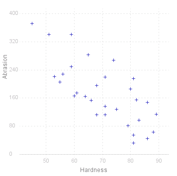
The response variable is "Abrasion". Suppose we're interested in seeing the influence of "Hardness" on "Abrasion", so we'll plot the values of Abrasion (along the y-axis) against the corresponding values of Hardness (along the x-axis). (Remember to include both MathymaStat.js and MathCasterGraph.js in the < head > section of the page):

< script type="text/javascript" src="../Lib/MathymaStat.js" >< /script >
< script type="text/javascript" src="../Lib/MathymaGraph.js" >< /script >
. . .
< p style="margin-left:20%" >
< script >
   myData.Plot("Abrasion:Hardness");
< /script >< /p >

(Note that we've already defined the data in the previous section, so this does not need to be done again.)

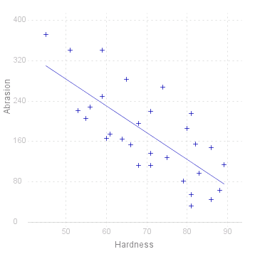
Plot has the ability to draw the best-fit straight line. To make it do this, the second argument must be set to true (note that there are no quote-marks, true is a JavaScript boolean literal, not a text string):

< p style="margin-left:20%" >
< script >
   myData.Plot("Abrasion:Hardness", true);
< /script >< p >

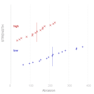
There is also a factor, "STRENGTH" in the data. It might be interesting to see if the Abrasion varies according to STRENGTH, so let's plot Abrasion for each level of STRENGTH:

< p style="margin-left:20%" >
< script >
   myData.Plot("Abrasion/Strength", true);
< /script >< p >

Note that when only one variable is plotted, the horizontal axis represents the value of the observation, and the values are distributed evenly along the vertical axis in ascending value, giving an empirical cumulate distribution function. The vertical lines that cross the plots indicate the mean values of each group of observations, and are only drawn if the second parameter (fit) is set to 'true'.

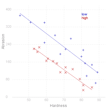
Finally, let's put the whole lot together, and see if the way Abrasion is affected by Hardness varies for the different levels of Strength:

< p style="margin-left:20%" >
< script >
   myData.Plot("Abrasion:Hardness/Strength", true);
< /script >< p >

---