Analysis of Variance
Anova Model
In an an #{AN}alysis #{O}f #{VA}riance model we look at some measure of the data known as the #~{response variable}, where the data is split up into groups or categories by properties known as #~{factors}. For example we might look into the height (response variable) of people depending on their country of origin (factor), or the output (resonse) of different machines (factor) also considiering the make of the machine (another factor).
Much of the theory for Anova is covered in the Probability and Statistics section of the notes. For a basic introduction see Linear Normal Models . For more advanced theory including multiple factor analysis see the Analysis of Variance notes.
Anova Example
The example we will use to illustrate the procedure is in fact looking at the output of machines on different days.
A factory producing building materials wants to research into the permeability of the produced materials. The number of seconds it takes for water to penetrate through the sheets of material is measured, and the logarithm of this number recorded . The production of three machines is looked into, and the experiment is conducted over nine days. Three measurements are taken for each machine on each day, giving a total of 81 observations. The finest factor is therefore one particular machine on a given day, this is known as the cross factor MACHINE*DAY.
Source: Anderson (1984)
The data is contained in the file MachineDay.xml, so the first thing we do is define the data and produce a summary. Note that we define three factors, DAY, MACHINE, and MACHINE*DAY. These are defined in two seperate AddFactor statements, but could as well have been defined in one statement, or three statements.
var myData = new mathyma.stats.DataBlock("StatsData/MachineDay.xml");
myData.ViewXML();
myData.AddVariables("PERM");
myData.AddFactors("MACHINE*DAY");
myData.AddFactors("DAY;MACHINE");
myData.Summary("PERM");
The factor structure in this example is fairly simple, but just to check that it's as we wanted we use the FactorStruct() method to print it out.
The variance table for the response variable (PERM) is then printed.
myData.FactorStruct();
myData.VarianceTable("PERM");
The information in the variance table can be used to test a number of hypotheses by specifying various models for the data. However MathymaStats can work out these figures automatically once you define a model.
The first model we will consider is where all three factors affect the response:
Model1 = myData.Model("PERM=MACHINE*DAY+MACHINE+DAY");
Model1.Display();
The figures in the Anova table above does not give us much information on which to make any decision about the data. The significance probability given, is that for testing the hypothesis that there is no variation in the data. As can be seen this is very low, so we can reject that possibility. As a starting point therefore we will adopt the model defined above as a basis on which to test further hypotheses.
The hypothesis we will look at is that there is no cross effect between machines and days, e.g. that a poorly performing machine will perform poorly whatever the day (statistically speaking of course - there will be variations). To do this we remove the cross factor MACHINE*DAY from the model. The model now only depends on the main factors MACHINE and DAY seperately. This is known as an additive model:
Model2 = myData.Model("PERM=MACHINE+DAY");
Model2.Display();
Note that as we have removed a factor, a portion of the sum of squares has moved to the residual (the total sum of squares remains constant). Given our starting point in the first model is it reasonable to accept that there is no cross effect between machines and days? We test this by seeing the effect of the model reduction ( see notes on Hypothesis Testing for some of the theory).
myData.ModelReduction(Model1,Model2);
The F-value is calculated as the ratio of the mean square for the reduction against the mean square for the original model. This is tested against an F-distribution with 16 and 54 degrees of freedom, giving a significance probability of about 15%, which is sufficient to accept the reduced model (using a standard test level of 5%).
Mathyma can be then be used to test further models (DAY only or MACHINE only).
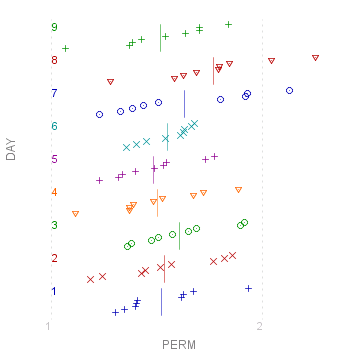
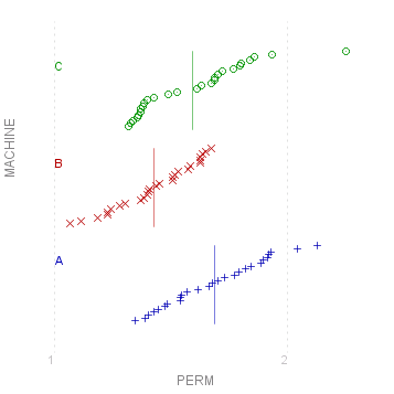
Finally we will plot the response variables against the two main factors.
myData.Plot("PERM/DAY",true);
myData.Plot("PERM/MACHINE",true);
  |
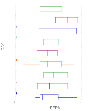
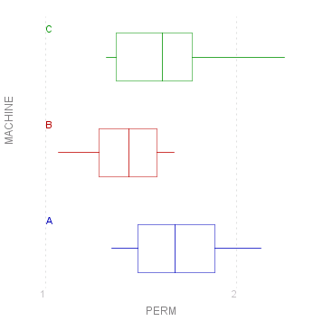
As you can see with the plot for "Day", with so many levels and so few observations, the scatter plot can be quite unclear. It is in such circumstances that a box-plot comes into its own:
myData.BoxPlot("PERM/DAY");
myData.BoxPlot("PERM/MACHINE");
  |
Source for the graphs shown on this page can be viewed by going to the diagram capture page .